
As promised in my previous blog, this is your next guide to understanding the basics of sentiment analysis on text documents and how to extract their hidden emotions 🙂
Technical foundation for this blog comes from DataCamp’s Sentiment Analysis in R.
Welcome to the World of Lexicons 💡
While doing my research on sentiment mining, I became acquainted with the important concept of subjective lexicons. The application of a lexicon is one of the two main approaches to sentiment analysis. It involves calculating sentiment from the semantic orientation of the words or phrases occurring in a text.
Available Lexicons in R:
➡ qdap’s polarity() function: uses a lexicon from hash_sentiment_huliu (U of IL @CHI Polarity (+/-) word research)
➡ tidytext: has a sentiments tibble with over 23,000 terms from three different subjectivity lexicons with these corresponding definitions:
| Word | Sentiment | Lexicon | Score |
|---|---|---|---|
| abhorrent | NA | AFINN | -3 |
| cool | NA | AFINN | 1 |
| congenial | positive | BING | NA |
| enemy | negative | BING | NA |
| ungrateful | anger | NRC | NA |
| sectarian | anger | NRC | NA |
➡ Principle of Least Effort which makes a limited lexicon library useful.
➡ You can always modify a lexicon based on your requirement!
Now, let’s get our hands dirty!
1. Defining the Business Problem
This is my favourite and most important step for the success of any project: asking the right questions. Some domain understanding or interaction with domain experts really helps in defining an appropriate problem statement.
You should be well aware of your data and have strong reasons to go for sentiment mining and not just because it sounds cool! 😉
For example, often in surveys, consumers are asked to rate a product on a certain scale. In such cases, an ordinal rating is good enough to determine consumer sentiment about the product, and sentiment analysis here would just be overkill. If you want to know what the consumer liked or disliked about the product, use an open-ended question and use the responses to extract meaningful insights.
In this blog, we shall find out which housing properties (e.g., proximity of restaurants, subway stations, hygiene, safety, etc.) lead to a good rental experience based on overall customer reviews.
2. Identifying Text Sources
One of the popular ways to extract customer reviews from any website is through webscraping. It can be done either in R or Python. I will keep this topic for my next blog. For now, I have chosen a dataset with 1,000 user reviews of AirBnB rentals in Boston.
Note: If you want to get a feel for webscraping in R, do read @jakedatacritic‘s article.
# Upload dataset in R (available as .rds file)
> bos_reviews <- readRDS("bos_reviews.rds", refhook = NULL)

3. Organizing and Cleaning the Text
In this step, we shall use two different lexicons (Polarity and BING) to determine the sentiment score for the collected housing reviews.
Simple Qdap-based Polarity score
It is a reasonable approach to begin with conducting sentiment analysis, as it familiarizes you with the data and helps set expectations to better address the business problem. For this purpose, the polarity function from the qdap package is really useful. It allows us to classify text as positive or negative.
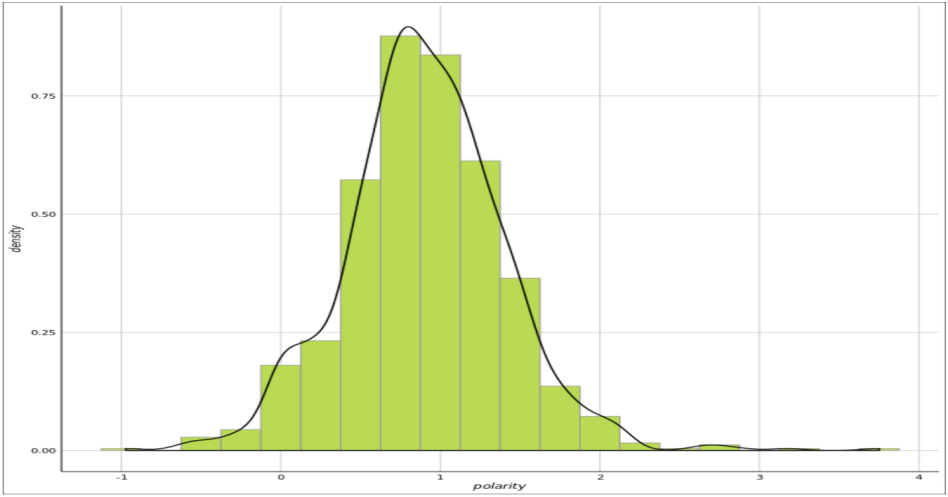
# Check out the boston reviews polarity overall polarity score
> bos_pol <- polarity(bos_reviews)
> bos_pol
 all total.sentences total.words ave.polarity sd.polarity stan.mean.polarity
 all       1000         70481       0.902         0.502          1.799

# Summary for all reviews
> summary(bos_pol$all$polarity)
 Min.    1st Qu.     Median     Mean     3rd Qu.     Max.     NA's
-0.9712   0.6047     0.8921    0.9022    1.2063    3.7510      1

# Kernel density plot of polarity score for all reviews
> ggplot(bos_pol$all, aes(x = polarity, y = ..density..)) + theme_gdocs() + geom_histogram(binwidth = 0.25, fill = "#bada55", colour = "grey60") +
 geom_density(size = 0.75)
TidyText’s BING Lexicon
Here, we will create the word data directly from the review column called ‘comments.’
> library(tidytext)
> library(tidyr)
> library(dplyr)

# Use unnest_tokens to make text lowercase & tokenize reviews into single words.
> tidy_reviews <- bos_reviews %>% unnest_tokens(word, comments)

# Group by and mutate to capture original word order within each group of a corpus.
> tidy_reviews <- tidy_reviews %>% group_by(id) %>% mutate(original_word_order = seq_along(word))

# Quick review
> tidy_reviews
A tibble: 70,834 x 3
Groups: id [1,000]
 id    word     original_word_order
 1 1   my         1
 2 1   daughter   2
 3 1   and        3
 4 1   i          4
 5 1   had        5
 6 1   a          6
 7 1   wonderful  7
 8 1   stay       8
 9 1   with       9
10 1   maura      10
# ... with 70,824 more rows

# Load stopwords lexicon
> data("stop_words")

# Perform anti-join to remove stopwords
> tidy_reviews_without_stopwords <- tidy_reviews %>% anti_join(stop_words)

# Getting the correct lexicon
> bing <- get_sentiments(lexicon = "bing")

# Calculating polarity for each review
> pos_neg <- tidy_reviews_without_stopwords %>%
inner_join(bing) %>%
count(sentiment) %>%
spread(sentiment, n, fill = 0) %>%
mutate(polarity = positive - negative)

# Checking outcome
> summary(pos_neg)
id                 negative          positive          polarity
Min. : 1.0       Min. : 0.0000      Min. : 0.00      Min. :-11.000
1st Qu.: 253.0  1st Qu.: 0.0000    1st Qu.: 3.00     1st Qu.: 2.000
Median : 498.0  Median : 0.0000     Median : 4.00    Median : 4.000
Mean : 500.4     Mean : 0.6139      Mean : 4.97      Mean : 4.356
3rd Qu.: 748.0  3rd Qu.: 1.0000     3rd Qu.: 7.00    3rd Qu.: 6.000
Max. :1000.0      Max. :14.0000      Max. :28.00      Max. : 26.000

# Kernel density plot of Tidy Sentiment score for all reviews
> ggplot(pos_neg, aes(x = polarity, y = ..density..)) + geom_histogram(binwidth = 0.25, fill = "#bada55", colour = "grey60") +
 geom_density(size = 0.75)

4. Creating a Polarity-Based Corpus
After the polarity check, we need to create a big set of text to use for the feature extraction in the following step.
a. Segregate all 1,000 comments into positive and negative comments based on their polarity score calculated in Step 2.
# Add polarity column to the reviews
> bos_reviews_with_pol <- bos_reviews %>% mutate(polarity = bos_pol$all$polarity)

# Subset positive comments based on polarity score
> pos_comments <- bos_reviews_with_pol %>% filter(polarity > 0) %>% pull(comments)

# Subset negative comments based on polarity score
> neg_comments <- bos_reviews_with_pol %>% filter(polarity < 0) %>% pull(comments)
b. Collapse the positive and negative comments into two larger documents.
# Paste and collapse the positive comments
> pos_terms <- paste(pos_comments, collapse = " ")

# Paste and collapse the negative comments
> neg_terms <- paste(neg_comments, collapse = " ")

# Concatenate the positive and negative terms
> all_terms <- c(pos_terms, neg_terms)
c. Create a Term Frequency Inverse Document Frequency (TFIDF) weighted Term Document Matrix (TDM).
Here, instead of calculating the frequency of words in the corpus, the values in the TDM are penalized for overused terms, which helps reduce non-informative words.
# Pipe a VectorSource Corpus
> all_corpus <- all_terms %>% VectorSource() %>% VCorpus()

# Simple TFIDF TDM
> all_tdm <- TermDocumentMatrix(all_corpus, control = list(
weighting = weightTfIdf,
removePunctuation = TRUE,
stopwords = stopwords(kind = "en")))

# Examine the TDM
> all_tdm
<> Non-/sparse entries: 4348/5582
Sparsity: 56%
Maximal term length: 372
Weighting: term frequency - inverse document frequency (normalized) (tf-idf)

# Matrix
> all_tdm_m <- as.matrix(all_tdm)

# Column names
> colnames(all_tdm_m) <- c("positive", "negative")
5. Extracting the Features
In this step, we shall extract the key housing features from the TDM, leading to positive and negative reviews.
# Top positive words
> order_by_pos <- order(all_tdm_m[, 1], decreasing = TRUE)

# Review top 10 positive words
> all_tdm_m[order_by_pos, ] %>% head(n = 10)
DocsTerms      positive     negative
 walk        0.004565669       0
 definitely  0.004180255       0
 staying     0.003735547       0
 city        0.003290839       0
 wonderful   0.003112956       0
 restaurants 0.003053661       0
 highly      0.002964720       0
 station     0.002697895       0
 enjoyed     0.002431070       0
 subway      0.002401423       0

# Top negative words
> order_by_neg <- order(all_tdm_m[, 2], decreasing = TRUE)

# Review top 10 negative words
> all_tdm_m[order_by_neg, ] %>% head(n = 10)
DocsTerms        positive     negative
 condition          0            0.002162942
 demand             0            0.001441961
 disappointed       0            0.001441961
 dumpsters          0            0.001441961
 hygiene            0            0.001441961
 inform             0            0.001441961
 nasty              0            0.001441961
 safety             0            0.001441961
 shouldve           0            0.001441961
 sounds             0            0.001441961
6. Analyzing the Features
Let’s compare the house features that received positive vs. negative reviews via WordClouds.
a. Comparison Cloud
> comparison.cloud(all_tdm_m,
max.words = 20,
colors = c("darkblue","darkred"))

b. Scaled Comparison Cloud
With this visualization, we shall fix the effect of grade inflation on the polarity scores of rental reviews before we perform the corpus subset by scaling review scores back to zero. This means some of the previously positive comments may become part of the negative subsection, or vice versa, since the mean is changed to zero.
# Scale/center & append
> bos_reviews$scaled_polarity <- scale(bos_pol$all$polarity)

# Subset positive comments
> pos_comments <- subset(bos_reviews$comments, bos_reviews$scaled_polarity > 0)

# Subset negative comments
> neg_comments <- subset(bos_reviews$comments, bos_reviews$scaled_polarity < 0)

# Paste and collapse the positive comments
> pos_terms <- paste(pos_comments, collapse = " ")

# Paste and collapse the negative comments
> neg_terms <- paste(neg_comments, collapse = " ")

# Organize
> all_terms<- c(pos_terms, neg_terms)

# VCorpus
> all_corpus <- VCorpus(VectorSource(all_terms))

# TDM
> all_tdm <- TermDocumentMatrix(
 all_corpus,
 control = list(
 weighting = weightTfIdf,
 removePunctuation = TRUE,
 stopwords = stopwords(kind = "en")))

# Column names
> all_tdm_m <- as.matrix(all_tdm)
> colnames(all_tdm_m) <- c("positive", "negative")

# Comparison cloud
> comparison.cloud(all_tdm_m,
 max.words = 100,
 colors = c("darkblue", "darkred"))

Besides the above analysis, I also wanted to assess the correlation between the efforts an author gives when writing positive reviews vs. negative reviews. This is done by plotting the word count of positive vs. negative comments.
# Create effort
> effort <- tidy_reviews_without_stopwords %>% count(id)

# Inner join
> pos_neg_with_effort <- inner_join(pos_neg, effort)

# Review
> pos_neg_with_effort
  A tibble: 953 x 5
  Groups: id [?]
 id      negative   positive   polarity   n

 1 1         0           4        4       26
 2 2         0           3        3       27
 3 3         0           3        3       16
 4 4         0           6        6       32
 5 5         0           2        2       8
 6 6         0           3        3       21
 7 7         0           5        5       18
 8 8         0           2        2       10
 9 9         0           4        4       12
10 10        1          15       14       46
# ... with 943 more rows

# Add pol
> pos_neg_pol <- pos_neg_with_effort %>% mutate(pol = ifelse(polarity >= 0,
 "Positive", "Negative"))

# Plot
> ggplot(pos_neg_pol, aes(polarity,n, color = pol)) +
 geom_point(alpha = 0.25) + geom_smooth (method = "lm", se = FALSE) + ggtitle("Relationship between word effort & polarity")

7. Drawing Conclusions
It’s not surprising the top positive terms included:
- walk
- well equipped
- restaurants
- subway
- stations
In contrast, the top negative terms included:
- automated posting
- dumpsters
- dirty
- hygiene
- safety
- sounds
Also, it can be seen that the author would spend more efforts in writing a stronger positive or negative review. How true is that!
I am sure with a larger dataset, we could mine deeper insights than we achieved with this small case study.
Thank you so much for reading!
My intention in writing this blog was to share the basic concepts of sentiment analysis with all of you aspiring data scientists, but we CAN’T stop here! I think I’m ready for a more elaborate emotion mining project for my portfolio 😀 How about you?
Do share your ideas/feedback in the comments below.
You can also connect with me on Linkedin.
Keep coding. Cheers!

Nice Share… thanks
LikeLike
Great effort. Have you tried applying this approach using ngram tokens?
LikeLike
In the first word cloud, it looks like the word “condition” is listed as a negative word. I’m curious, as to why that is? Is it because of the frequency of its use in a negative context, or is it simply classified as such in one of the lexicons mentioned (or is there another reason)?
LikeLike
It is primarily because of the way word is categorized in the lexicon.
LikeLike
Amazing work! Both insightful and inspiring. Thank you for sharing.
LikeLike
Pingback: Text Mining and Sentiment Analysis with Canadian Underwriter Magazine Headlines – datacritics
Thanks! Glad you found the article helpful.
LikeLike