Using Data Science to Help Win Fantasy Football Games

A couple years into my first fantasy football league, I felt the need to track game statistics to find hidden value in players. I was in a pretty competitive head-to-head league with fourteen members or ‘team managers’ who are able to carry over three players into the next season, and most trades are vetoed by division rivals if they were even proposed.

If you’re not familiar with fantasy football, that just means there were more teams than usual, keeping more top-tier players than usual year-over-year.

This made for an environment where top performing players were hard to come by. One would need to make accurate predictions on college players’ 2-3 year NFL outlooks to draft them on their rookie year in the league. I don’t follow college football and even the experts who do sometimes have trouble predicting rookies’ level of success in the NFL.

This is where I turned to statistics for help about 8 years ago – copying and pasting from Yahoo! Sports to my Excel spreadsheet and analyzing the data in there. I primarily used this data analysis to find favourable matchups where average to 2^nd tier players can produce 1^st tier results. Other ways this analysis could help in your fantasy football league will also be touched on later in the article. For now, here’s what’s under the hood.

 

I built a solution to web-scrape weekly statistics using Python, then synthesize the data with R and present the output via a Shiny app. You can read about my Python web-scraping work here. The rest of this article will go through the data work in R. All Python and R code can be found in my GitHub repository and the Shiny app can be found here. [EDIT: Latest Update]

Cleaning the Scraped Raw Data

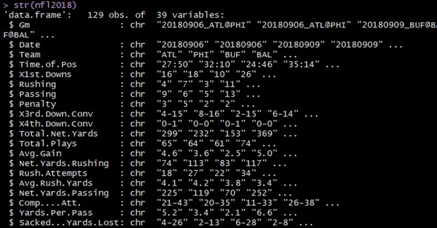
The scraped data imported to R was originally all in character format, and some of the field names just came through funny. Clean up was required and mainly consisted of:

• Explicitly renaming field names
• Setting appropriate data types like times, dates and numbers
• Splitting fractions into separate numerator and denominator fields themselves.
  (For example, completed passes of attempted passes by the QB was originally expressed as ’19-29′. This was split into 19 completed and 29 attempted, in separate fields)

Producing More Game Statistics

This brings me to the first distinction I think my analysis approach has – tracking all ‘stats allowed’. For a given game I’m documenting, all of an opponent’s stats is copied to the team at question, making an easy side-by-side comparison of all the stat categories the team produced and allowed.

To illustrate, consider the screenshot just above: Time of Possession (TOP) when earned by the opponent is also captured as Time on Defense (TOD) for the other team. TotalPlays by Philadelphia copied as PlaysDefended by Atlanta. Yards Allowed, Rushes Defended, Rushing Yards Allowed, etc.

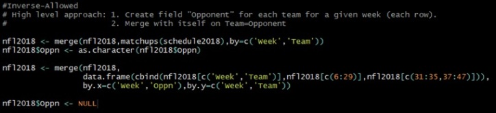
Below is the code I used to achieve this.

This is distinctive because there’s now readily available capability to compare how a team’s defensive squad is doing with how their opposing offensive squad is doing for past given weeks on every stat category.

Capturing Recent Performance

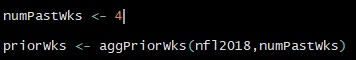
Typical statistics tables online report on the total season thus far. Teams’ performance may differ substantially between September and November. My approach only extracts recent weeks from the annual data set, and the user has an opportunity here to define how far back to include in the analysis.

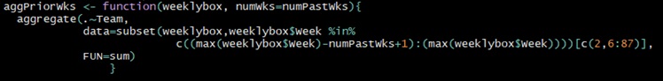
Due to bye weeks, not every team plays the same number of games as the number of weeks. Since I do want to calculate touchdowns per game, and not touchdowns per week, I’ll need to build Games Played into my data set.

I then proceeded to build the metrics on recent performance, which will be used to predict current week outcomes and recommend match-ups to take advantage of.

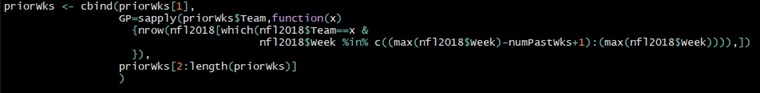
To merge the historical data with the current week’s team match-ups, I started with building a table containing each team and who they’re playing.

To that table, I appended the team pairs’ various metrics as a function of how one team’s doing and how their opponent has been defending.

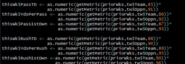
You’ll notice here that I chose to multiply a team’s offensive performance by their opponent’s defensive performance. This function was just what I came up with quickly. Here’s the thought behind it, and you can apply this to many other sports too:

If a team is scoring a lot of points, yards, touchdowns or goals, I like a match-up where their opponent is also giving up a lot of the same. So creating a pair-wise variable by multiplying the two features was the operation I ran with for now to ensure such scenarios were highlighted by the numbers.

For the last two steps, I ranked the teams’ metrics…

…and took average ranks of metric groups that were common to a particular fantasy football position.

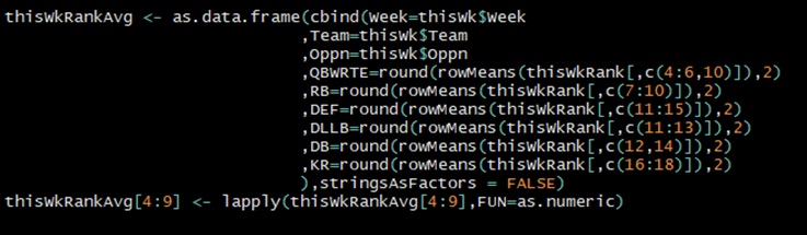
Take for example ‘QBWRTE‘. This is quarterbacks, wide-receivers and tight-ends – all the positions which would primarily benefit from an advantageous passing match-up. This takes the average ranking of columns 4, 5, 6 and 10: PassTD, YdsPerPass, Pass1stDwn and RZPctDiff.

PassTD is where the team ranked by number of passing touchdowns per game as of late, vs number of passing touchdowns their opponent allowed.

Yards per pass is used as oppose to yards per completion or yards per game because YPP takes completion rate and accuracy into account.

Passing 1st Downs is where the team ranked by the proportion of their 1st downs converted with a pass, vs the proportion allowed by their opponent.

RZPctDiff was a fascinating one I made up just over the course of this project. It’s an overall measure of a team’s ability to maintain possession in the red zone and either score a pass TD, rush TD or a field goal. Red zone percentage is the number of TDs or FGs a team scored divided by the number of times they were in the red zone. I compared a team’s RZ% achieved vs their opponent’s RZ% allowed, by subtracting the inverse of the RZ% allowed from the RZ% achieved. This way, the higher the achieved, and the higher allowed, the higher my final statistic.

The following are the rest of the definitions:

• RB – Running backs
• DEF – Defensive Team (project does not measure kick/punt returning yet)
• DLLB – Defensive Linemen and Linebackers. For IDP formats.
• DB – Defensive Backs. For IDP formats.
• KR – Kicker

Finally, this ranking table was presented using Shiny. Most of the credit here goes to the great folks that shared a plethora of templates for public use. I just subbed in my table names and inserted the existing code into my own project.

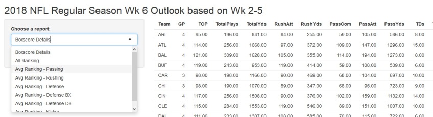
Boxscore Details and All Ranking will show all statistics measured and ranked. The Avg Ranking series are where average rankings by position of interest, sorted by the position selected in the drop down. (‘BX’ represents ‘box’, representing the area of the field where defensive linemen and linebackers line up.)

Interpreting the Charts

Here’s a walk through of some primary intended uses. We’ll also see how the recommendations panned out for Week 6.

Who to Start/Bench

Quarterbacks, Receivers and Tight Ends

“Avg Ranking – Passing” is saying ATL and TB both have a favourable passing match-up against one another. In other words, both teams have been performing well in the passing attack and both have not defended it well.

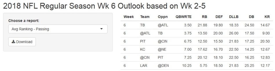
The average ranking of the above mentioned passing touchdowns per game, yards per pass attempt, passing 1st down proportion and overall red zone scoring percentage pair-wise variables is between 3rd and 4th out of 30 teams playing.

The actual outcome: Four of the top five QB performances this week aligned with the analysis. Further data analysis on receiver and tight end targets and snap counts is required to predict which one(s) of the 3 to 4 pass catchers will benefit most from the QB’s success. For now, within the scope of this article, the QB for TB, ATL, PIT and KC were predicted to have strong performances and did.

Running backs

The rushing (RB) prediction did not fare as well. The LA Rams (Todd Gurley) were predicted to have a strong rushing game and actually did. However Todd Gurley produces those numbers regularly, regardless of the match-up (aka “match-up proof”). In fact he has earned the nickname “God Gurley” in the fantasy football community as of late. However; even though SEA and NE did not have individual RBs that made the top 5 list, their RBs combined had pretty strong outings. Seattle and New England utilized 3 separate RBs each to produce 123 (4.2 yards per carry) and 161 (4.9 YPC) yards respectively. In real football, rushing for anything over 3.4 YPC (10 yds / 3 downs) is a winning ingredient. Again, also utilizing RB snap count stats would provide a heads up on these scenarios where a team will rotate between RBs.

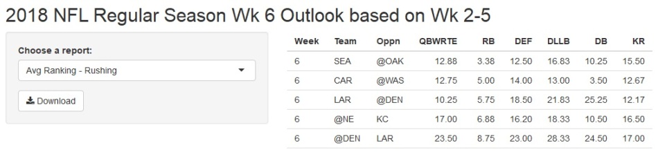
The actual outcome: One of the top five RB performances this week aligned with the analysis. Two required more analysis to interpret and use appropriately, and two were just false positives.

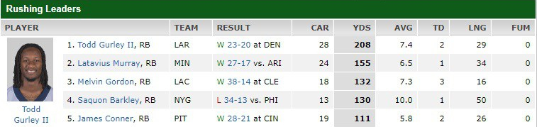
Lastly on RBs, Latavius Murray (MIN) and Saquon Barkley (NYG) held low-average expectations in week 6 and the analysis failed to predict their surprising success. MIN and NYG were ranked at the bottom of the RB list.

(Note: displayed stats from ESPN prior to Monday Night Football’s SF@GB match-up)

Other Concepts

When to Add/Drop/Trade

Each week team managers have an opportunity to modify their roster by adding players from the pool of players not already on a team (via free agency or waiver wire), or even trade players with other team managers.

Rosters can’t exceed a certain number of players so decisions must be made on who to let go in exchange. This analysis can be used to forecast how easy or hard players’ match ups are for the next several weeks.

The above walk-through analyzed week 6 match-ups based on week 2-5. I would also analyze week 7 or even week 8 match ups to forecast, and compose my roster with players with favourable match-ups for the next several weeks. In the past, I’ve been able to pick up players from waivers 1 or 2 weeks prior to media outlets recommending to add them for the immediate upcoming week. The idea of ‘renting’ a player for just one week’s performance can be risky so think carefully on who you let go – they get scooped up in the meantime.

Streaming

A little disclaimer here since you’ve read this far! I’ve never won a championship in my 8 year career. However in my many playoff disappointments, I lose to teams with “home run hitter” RBs and WRs. Seasoned team managers don’t need data science to know these are the key positions to win championships. With roster size and composition limitations, you only have so many spots on your roster to “stash” undervalued RBs and WRs to wait for them to flourish (or not).

Many team managers hold multiple QBs, TEs and Defensive personnel to cover for bye-weeks and open options for match-ups. I stopped doing that just a couple years ago and held the absolute minimum number of players at those positions so I could maximize my RBs and WRs stash. I covered for bye weeks and (highly) unfavourable match-ups by adding/dropping QBs and most defensive personnel on a weekly basis as needed. (I spent higher than usual draft picks on top TEs too.)

This approach of practically using the waiver wire as your bench is referred to as “streaming.” The analysis I was doing allowed me to pick and stash undervalued RBs and WRs, and find average/risky QBs and defenses that can secure enough points to be competitive on a weekly basis. On my last year in the 14 team league, I ended the year with Tyreek Hill and Stefon Diggs – both were WRs who didn’t score many points when I picked them up but these days, you can expect they’ll have a few games a year with 150+ yds and multiple TDs.

News & Media

One last note regarding timing – I found most pundits start making recommendations on Wednesday or Thursday as they spend Tuesday summarizing the past week and wait for reporters and beat writers to collect more intel from teams.

While this analysis is available immediately after the last game of the week, the best use of it is in tandem with the locker room news, injury reports and rumours the media provides. This is cautious so you don’t drop a player for another that’s on the wrong side of a “Questionable” injury status!

In conclusion

It’s a weekly grind in fantasy football, to which I found a rhythmic process to manage; collect and analyze data Sun/Mon/Tue night (there’s player and snap count data which I often use as well and did not get into yet), be the first by Wednesday morning to claim undervalued players from free agency for a pipeline of favourable match-ups, while hedging on as many RBs and WRs as possible with potential come playoffs.

I’d be curious to know how others are using quantitative analysis to set themselves up for success in fantasy football. I know there’s a play-by-play data set out there commonly worked on on Kaggle. Incorporating that data with this pair-wise team match-up data could uncover some fascinating insights. Are there better ways to create that pair-wise statistic aside from multiplying? Feel free to comment.